Working everyday gives you always a number of problems that you have to face it, and it was my case when I needed to make a list on excel to select a value that modifies a next list depending on the value selected.
The way I solved this inconvenient will be shown here with a simple example: there's a list of 3 countries and depending on the selected one, the next cell must show a list of some cities to be selected. Despite the example is performed in Excel 2010, I think that you can apply it even on Excel 2003.
Before beginning it's necessary to create a sheet which will contain our data base with the countries and the city-country relationship, then, we have to group the cities of a determined country in a named range. To do this, you only select the cities for Australia, for instance, and go to the cell that is on the left of the function bar and type there the name of the country and press Enter, thus, for every country.
Having the respective named ranges, go to the tab where the lists will be, select the cell which will show the country list and select "Data" ribbon (in the image I use a Spanish version of Excel), "Data Validation..." option .
Here, you have to select in the "Configuration" tab the "List" value under the "Allow:" section. Besides, you must put under "Source:" the range of the countries to be shown and press "OK".
That is how you build your first list, which is the easiest part.
It's time to set the second list and it's going to be different depending on the country selected in the previous cell. The procedure to be followed is the same, but in the "Source:" section you only have to use the INDIRECT function referring to the cell which contains the country selected.
This is how the second list will dynamically change together with the selected country, because when a country is selected, the second cell takes its name and using the function brings all the cities that are in the named range that had been established at the beginning.


Super duper cool.
ReplyDeleteHi Ronald, I am trying to use this formula, but its not working, somehow following the same steps with my excel 2010, gives me an error.
ReplyDeleteHow does the indirect formula know where to get the data that it brings?
Hi Daniel! indirect function just convert a text given as parameter into a reference, I mean, if you write this =indirect("A1"), the function will bring the value which is in the reference A1.
DeleteTherefore, when I show =indirect(B3), Excel will derive =indirect("Australia") because B3 contains the string "Australia". But as "Australia" is a named range then Excel brings all the values which are inside "Australia" range.
Hello! I was experiencing quite the same problem which I partially solved using your method. However I would like to adjust it a little (if possible). My problem is that the first list (in A1) has just values YES or NO. When I select NO, in the B1 there should be a list of given dates. So far this works great, but when I select YES, I want to have an exact value in the B1 (specificaly 1.1.2013) instead of having another list with this single value. Is there any way of doing that? Thank you for any response!
ReplyDeleteHi! sorry for being late, maybe this could help you, on B1 you should use a data validation using lists, using this function:
Delete=IF(A1="YES",INDIRECT("UNIQUE_VALUE_LIST"),INDIRECT("MULTIPLE_VALUE_LIST"))
Yes, you need to have a named range "UNIQUE_VALUE_LIST" and "MULTIPLE_VALUE_LIST".
I got the error message too and said yes, continue. What happens is the second column will not show a list until you select a country in the first column. Once you select a country, it works like a charm!
ReplyDeleteHi! I didn't understand what you're trying to explain... I'll appreciate if you could give me more details. Thanks.
DeleteDude, that is sweet! Worked like a charm. Good job!
ReplyDeleteThanks a lot! : )
Delete